Week of December 9, 2019

Normal Distribution

Data can be "distributed" (spread out) in different ways.

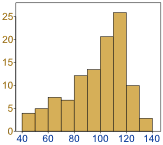
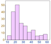
It can be spread out more on the left		Or more on the right

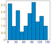
Or it can be all jumbled up

But there are many cases where the data tends to be around a central value with no bias left or right, and it gets close to a "Normal Distribution" like this:

A Normal Distribution

The "Bell Curve" is a Normal Distribution.
And the yellow histogram shows some data that
follows it closely, but not perfectly (which is usual).

It is often called a "Bell Curve" because it looks like a bell.

Many things closely follow a Normal Distribution:

• heights of people
• size of things produced by machines
• errors in measurements
• blood pressure
• marks on a test

We say the data is "normally distributed":

The Normal Distribution has:

• mean = median = mode
• symmetry about the center
• 50% of values less than the mean
  and 50% greater than the mean

Quincunx

You can see a normal distribution being created by random chance! It is called the Quincunx and it is an amazing machine. Have a play with it!

Standard Deviations

The Standard Deviation is a measure of how spread out numbers are (read that page for details on how to calculate it).

When we calculate the standard deviation we find that generally:

68% of values are within 1 standard deviation of the mean 95% of values are within 2 standard deviations of the mean 99.7% of values are within  3 standard deviations of the mean

Example: 95% of students at school are between 1.1m and 1.7m tall.

Assuming this data is normally distributed can you calculate the mean and standard deviation?
The mean is halfway between 1.1m and 1.7m:

Mean = (1.1m + 1.7m) / 2 = 1.4m

95% is 2 standard deviations either side of the mean (a total of 4 standard deviations) so:

1 standard deviation	= (1.7m-1.1m) / 4
	= 0.6m / 4
	= 0.15m

And this is the result:

It is good to know the standard deviation, because we can say that any value is:

• likely to be within 1 standard deviation (68 out of 100 should be)
• very likely to be within 2 standard deviations (95 out of 100 should be)
• almost certainly within 3 standard deviations (997 out of 1000 should be)

Standard Scores

The number of standard deviations from the mean is also called the "Standard Score", "sigma" or "z-score". Get used to those words!

Example: In that same school one of your friends is 1.85m tall

You can see on the bell curve that 1.85m is 3 standard deviations from the mean of 1.4, so:

Your friend's height has a "z-score" of 3.0

It is also possible to calculate how many standard deviations 1.85 is from the mean
How far is 1.85 from the mean?

It is 1.85 - 1.4 = 0.45m from the mean

How many standard deviations is that? The standard deviation is 0.15m, so:

0.45m / 0.15m = 3 standard deviations

So to convert a value to a Standard Score ("z-score"):

• first subtract the mean,
• then divide by the Standard Deviation

And doing that is called "Standardizing":

We can take any Normal Distribution and convert it to The Standard Normal Distribution.

Example: Travel Time

A survey of daily travel time had these results (in minutes):

26, 33, 65, 28, 34, 55, 25, 44, 50, 36, 26, 37, 43, 62, 35, 38, 45, 32, 28, 34

The Mean is 38.8 minutes, and the Standard Deviation is 11.4 minutes (you can copy and paste the values into the Standard Deviation Calculator if you want).
Convert the values to z-scores ("standard scores").

To convert 26:

first subtract the mean: 26 - 38.8 = -12.8,

then divide by the Standard Deviation: -12.8/11.4 = -1.12

So 26 is -1.12 Standard Deviations from the Mean

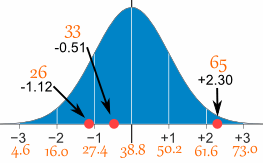
Here are the first three conversions

Original Value	Calculation	Standard Score (z-score)
26	(26-38.8) / 11.4 =	-1.12
33	(33-38.8) / 11.4 =	-0.51
65	(65-38.8) / 11.4 =	+2.30
...	...	...

And here they are graphically:

You can calculate the rest of the z-scores yourself!

Here is the formula for z-score that we have been using:

z is the "z-score" (Standard Score) x is the value to be standardized μ is the mean σ is the standard deviation

Why Standardize ... ?

It can help us make decisions about our data.

Example: Professor Willoughby is marking a test.

Here are the student's results (out of 60 points):

20, 15, 26, 32, 18, 28, 35, 14, 26, 22, 17

Most students didn't even get 30 out of 60, and most will fail.
The test must have been really hard, so the Prof decides to Standardize all the scores and only fail people 1 standard deviation below the mean.
The Mean is 23, and the Standard Deviation is 6.6, and these are the Standard Scores:

-0.45, -1.21, 0.45, 1.36, -0.76, 0.76, 1.82, -1.36, 0.45, -0.15, -0.91

Now only 2 students will fail (the ones lower than −1 standard deviation)
Much fairer!

It also makes life easier because we only need one table (the Standard Normal Distribution Table), rather than doing calculations individually for each value of mean and standard deviation.

Source:https://www.mathsisfun.com/data/standard-normal-distribution.html